Anacode Toolkit
This library is a helper tool for users of the Anacode Web&Text API, a REST API for Chinese web data collection and Natural Language Processing. The following operations are possible with the library:
- Abstraction of HTTP protocol that is used by Anacode Web&Text API. Besides, concurrent API querying is made simple.
- Conversion of JSON analysis results into flat table structures.
- Common aggregation and selection tasks that can be performed on API analysis results, like finding the most discussed concepts or ten best-rated entities
- Convenient plotting functions for aggregated results, ready to use in print documents.
The first two features are covered by the module anacode.api; 3. and 4. are covered by anacode.agg.
Installation
The library is published via PyPI and works on python2.7 and python3.3+. To install from PyPI simply use pip:
pip install anacode
You can also clone its repository and install from source using the setup.py script:
git clone https://github.com/anacode/anacode-toolkit.git
cd anacode-toolkit
python setup.py install
Using Anacode API and saving results (anacode.api)
Querying the API
The anacode.api module provides functionality for http communication with the Anacode Web&Text API.
The class anacode.api.client.AnacodeClient can be used to analyze Chinese texts.
>>> from anacode.api import client
>>> # base_url is optional
>>> api = client.AnacodeClient(
>>>     'token', base_url='https://api.anacode.de/')
>>> # this will create an http request for you, send it to appropriate
>>> # endpoint, parse the result and return it in a python dict
>>> json_analysis = api.analyze(['储物空间少', '后备箱空间不小'], ['concepts'])
There is also a class anacode.api.client.Analyzer to perform bulk querying. It can used
multiple threads and saves the results either to pandass
dataframes or csv files. However, it is not intended for direct usage - instead, please
use the interface to it that is covered in Using analyzer.
Saving results
Since there is no analysis tool that can analyse arbitrary json schemas well,
the toolkit offers a simple way to convert lists of API JSON results to a standard SQL-like
data structure. There are two possibilities: you can convert your output to a
pandas.DataFrames
or store it to disk in csv files, making it ready to be input into various
data processing programs such as Excel. The JSON > CSV conversion code lives in
anacode.api.writers. You are not expected to use it directly, but here is
quick example how to load sentiment analysis results into memory as a dataframe.
>>> from anacode.api import writers
>>> sentiment_json_output_0 = [
>>>     {"sentiment_value": 0.7},
>>>     {"sentiment_value": -0.1},
>>> ]
>>> sentiment_json_output_1 = [
>>>     {"sentiment_value": 0.34},
>>> ]
>>> df_writer = writers.DataFrameWriter()
>>> df_writer.init()
>>> df_writer.write_sentiment(sentiment_json_output_0)
>>> df_writer.write_sentiment(sentiment_json_output_1)
>>> df_writer.close()
>>> df_writer.frames['sentiments']
   doc_id  text_order  sentiment_value
0       0           0             0.7
1       0           1            -0.1
2       1           0             0.34
The schemas of the tables are described in Table schema.
Both anacode.api.writers.DataFrameWriter and
anacode.api.writers.CSVWriter have the same interface. They
generate document ids (doc_id) incrementally and separately for analyze
and scrape. That means that document id gets incremented each time you
successfully receive an analysis/scrape result from API.
Using analyzer
If you want to analyze a larger number of texts and store
the analysis results to a csv file, you can use the
anacode.api.client.analyzer() function. It provides an easy interface to
bulk querying and storing results in a table-like data structure.
The following code snippet analyses categories and sentiment for all documents
in a single thread by bulks of size 100 and saves the resulting csv files to the folder
ling/.
>>> from anacode.api import client
>>> documents = [
>>>     ['Chinese text 1', 'Chinese text 2'],
>>>     ['...'],
>>> ]
>>> with client.analyzer('token', 'ling') as api:
>>>     for document in documents:
>>>         api.analyze(document, ['categories', 'sentiment'])
By contrast, below code snippet analyses categories and sentiment for all documents in two threads by bulks of size 200 and saves the output as pandas DataFrames to provided dictionary.
>>> from anacode.api.client import analyzer
>>> documents = [
>>>     ['Chinese text 1', 'Chinese text 2'],
>>>     ['...'],
>>> ]
>>> output_dict = {}
>>> with analyzer('token', output_dict, threads=2, bulk_size=200) as api:
>>>     for document in documents:
>>>         api.analyze(document, ['categories', 'sentiment'])
>>> print(output_dict.keys())
dict_keys(['concepts', 'concepts_surface_strings', 'sentiments'])
Single document mode
Anacode API supports sending list of texts in two different modes. By default
each text from list is considered to be one separate document. This means that
categories and sentiment analysis are applied for each text from the list
separately. You can make Anacode API consider texts as parts of one document
by setting single_document switch of
analyze. This will result in
server performing just one categories and just one sentiment analysis on all
the texts together. You can read about this behavior in
API documentation.
On Anacode Toolkit side of things setting single_document mode will result in text_order being used to mark different paragraphs of the bigger document in csv and DataFrame output of analysis.
Aggregation framework (anacode.agg)
Data loading
The Anacode Toolkit provides the anacode.agg.aggregation.DatasetLoader for
loading analysed data from different formats:
From analysis result of API
If you have either result dictionary from anacode API or list of these results you can load them to memory using
DatasetLoader.from_api_result.>>> from anacode.agg import DatasetLoader >>> from anacode.api import client >>> api = client.AnacodeClient('<your token>') >>> result1 = api.analyze(['...'], analyses=['concepts']) >>> single_result_dataset = DatasetLoader.from_api_result(result1) >>> result2 = api.analyze(['...'], analyses=['concepts']) >>> whole_result_dataset = DatasetLoader.from_api_result([result1, result2])
Path to folder with csv files
If you stored the analysis results in csv files (using
anacode.api.writers.CSVWriter), you can provide the path to their parent folder toDatasetLoader.from_pathto load all available results. If you want to load older backed-up csv files, you can use backup_suffix argument of the method to specify suffix of files to load.From
anacode.api.writers.WriterinstanceIf you used an instance of Writer (either DataFrameWriter or CSVWriter) to store the analysis results, you can pass a reference to it to the
DatasetLoader.from_writerclass method.From
pandasdataframesYou can also use DatasetLoader‘s
DatasetLoader.__init__which simply takes an iterable of pandas.DataFrame objects with analyzed data.
Accessing analysis data
There are two ways to access the analysis results from
DatasetLoader. First, you can access
pandas.DataFrame directly using
DatasetLoader.__getitem__, as
follows: absa_texts = dataset[‘absa_normalized_texts’]. The format of these
data frames is described below. Second, you can get higher-level access to the separate datasets via
DatasetLoader.categories,
DatasetLoader.concepts,
DatasetLoader.sentiments or
DatasetLoader.absa.
The latter returns anacode.agg.aggregation.ApiCallDataset instances
and actions you can perform with it will be explained in the next chapter.
Text order field
In all calls documentation you can notice that they take not a single text for analysis but list of texts. Every call also returns list of analysis, one for each text given. text-order property in csv row defines index of analysis in this list that produced the row. That means that you can use text-order column to match analysis results to specific pieces of text that you sent to the API for analysis.
Table schema
In this section, we describe the table schema of the analysis results for each of the four calls.
Categories
categories.csv
categories.csv will contain one row per supported category name per text. You can find out more about category classification in its documentation
- doc_id - document id generated incrementally
- text_order - index to original input text list
- category - category name
- probability - float in range <0.0, 1.0>
The probabilities for all categories for a given text sum up to 1.
Concepts
concepts.csv
- doc_id - document id generated incrementally
- text_order - index to original input text list
- concept - name of concept
- freq - frequency of occurrences of this concept in the text
- relevance_score - relative relevance of the concept in this text
- concept_type - type of concept (cf. here for list of available concept types)
concept_surface_strings.csv
concept_surface_strings.csv extends concepts.csv with surface strings that were used in text that realize it’s concepts
- doc_id - document id generated incrementally
- text_order - index to original input text list
- concept - concept identified by anacode nlp
- surface_string - string found in original text that realizes this concept
- text_span - string index to original text where you can find this concept
Note that if concept is used multiple times in original text there will be multiple rows with it in this file.
Sentiment
sentiment.csv
- doc_id - document id generated incrementally
- text-order - index to original input text list
- sentiment_value - evaluation of document sentiment; values are from [-1,1]
ABSA
absa_entities.csv
- doc_id - document id generated incrementally
- text_order - index to original input text list
- entity_name - name of the entity
- entity_type - type of the entity
- surface_string - string found in original text that realizes this entity
- text_span - string index in original text where surface_string can be found
absa_normalized_text.csv
- doc_id - document id generated incrementally
- text_order - index to original input text list
- normalized_text - text with normalized casing and whitespace
absa_relations.csv
- doc_id - document id generated incrementally
- text_order - index to original input text list
- relation_id - since the absa relation output can have multiple relations, we introduce relation_id as a foreign key
- opinion_holder - optional; if this field is null, the default opinion holder is the author himself
- restriction - optional; contextual restriction under which the evaluation applies
- sentiment_value - polarity of evaluation, has values from [-1, 1]
- is_external - whether an external entity was defined for this relation
- surface_string - original text that generated this relation
- text_span - string index in original text where surface_string can be found
absa_relations_entities.csv
This table is extending absa_relations.csv by providing list of entities connected to evaluations in it.
- doc_id - document id generated incrementally
- text_order - index to original input text list
- relation_id - foreign key to absa_relations
- entity_type -
- entity_name -
absa_evaluations.csv
- doc_id - document id generated incrementally
- text_order - index to original input text list
- evaluation_id - absa evaluations output can rate multiple entities, this serves as foreign key to them
- sentiment_value - numeric value how positive/negative statement is; from [-1, 1]
- surface_string - original text that was used to get this evaluation
- text_span - string index in original text where surface_string can be found
absa_evaluations_entities.csv
- doc_id - document id generated incrementally
- text_order - index to original input text list
- evaluation_id - foreign key to absa_evaluations
- entity_type -
- entity_name -
Aggregations
The Anacode Toolkit provides set of common aggregations over the analysed
data. These are accessible from the four subclasses of
ApiCallDataset -
CategoriesDataset,
ConceptsDataset,
SentimentDataset and
ABSADataset. You can get any of those using
the corresponding properties of the class DatasetLoader
(categories,
concepts,
sentiments and
absa).
Here is a list of aggregations and some other convenience methods with descriptions and usage examples that can be performed for each api call dataset.
ConceptsDataset
concept_frequency(concept, concept_type='', normalize=False)Concepts are returned in the same order as they were in input.
>>> concept_list = ['CenterConsole', 'MercedesBenz',
>>>                 'AcceleratorPedal']
>>> concepts.concept_frequency(concept_list)
Concept
CenterConsole       27
MercedesBenz        91
AcceleratorPedal    39
Name: Count, dtype: int64
Limiting concept_type may zero out counts:
>>> concepts.concept_frequency(
>>>     concept_list, concept_type='feature')
Feature
CenterConsole       27
MercedesBenz         0
AcceleratorPedal    39
Name: Count, dtype: int64
The next two code samples demonstrate how percentages can change if concept_type filter changes.
>>> concepts.concept_frequency(concept_list, normalize=True)
Concept
CenterConsole       0.005560
MercedesBenz        0.018740
AcceleratorPedal    0.008031
Name: Count, dtype: float64
>>> concepts.concept_frequency(
>>>     concept_list, concept_type='feature', normalize=True)
Feature
CenterConsole       0.009174
MercedesBenz        0.000000
AcceleratorPedal    0.013252
Name: Count, dtype: float64
most_common_concepts(n=15, concept_type='', normalize=False)>>> concepts.most_common_concepts(n=3)
Concept
Automobile          533
BMW                 381
VisualAppearance    241
Name: Count, dtype: int64
Also read about concept_frequency to see how concept_type and normalize can change output.
least_common_concepts(n=15, concept_type='', normalize=False)>>> concepts.least_common_concepts(n=3)
Concept
30       1
Lepow    1
Lid      1
Name: Concept, dtype: int64
Also read about concept_frequency to see how concept_type and normalize can change output.
co_occurring_concepts(concept, n=15, concept_type='')>>> concepts.co_occurring_concepts('VisualAppearance', n=5, >>> concept_type='feature')
Feature
Interior    33
Body        26
Comfort     17
Space       17
RearEnd     16
Name: Count, dtype: int64
Also read about concept_frequency to see how concept_type can change output.
nltk_textcollection(concept_type='')Creates nltk.text.TextCollection containing concepts found by linguistic analysis.
make_idf_filter(threshold, concept_type='')Creates IDF filter from concepts found by linguistic analysis. You can read more about IDF filtering on many places, for your convenience we provide a link to stanford webpage.
make_time_series(concepts, date_info, delta, interval=None)You will have to provide date_info dictionary to this function. The keys of date_info correspond to consecutive integers; the values correspond to
datetime.dateobjects:>>> print(date_info)
{0: datetime.date(2016, 1, 1),
 1: datetime.date(2016, 1, 2),
 2: datetime.date(2016, 1, 3),
 3: datetime.date(2016, 1, 4),
 4: datetime.date(2016, 1, 5),
 5: datetime.date(2016, 1, 6),
 ...
}
When you are using scraped data from Anacode in json format you can build the dictionary by looping over documents with date field, parsing it and storing it in dictionary under index of the document like this:
>>> from datetime import datetime
>>> date_info = {}
>>> for index, doc in enumerate(scraped_json_data):
>>>     if not doc['date']:
>>>         continue
>>>     date_info[index] = datetime.strptime(d['date'], '%Y-%m-%d')
When you have date_info dictionary generating time series is simple. Keep in mind that resulting time series ticks include it’s starting date and exclude ending date. So a tick who starts at Start and ends at Stop will include these: Start <= concept’s document time < Stop.
>>> concepts.make_time_series(['Body'], date_info,
>>>                           timedelta(days=100))
    Count   Concept     Start       Stop
0   89      Body    2016-01-01  2016-04-10
1   25      Body    2016-04-10  2016-07-19
2   2       Body    2016-07-19  2016-10-27
3   3       Body    2016-10-27  2017-02-04
When you limit interval (start and stop of ticks) and you specify delta such that start + K * delta = stop cannot be solved the stop will stretch to the first following date for which the formula can be solved. For instance setting start to 2016-01-01 and stop to 2016-01-07 and delta to 4 days, stop will be changed to 2016-01-09.
>>> concepts.make_time_series(['Body'], date_info,
>>>                           timedelta(days=4),
>>>                           (date(2016, 1, 1), date(2016, 1, 7)))
    Count  Concept     Start      Stop
0   3      Body     2016-01-01   2016-01-05
1   2      Body     2016-01-05   2016-01-09
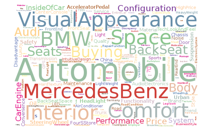
concept_cloud(path, size=(600, 350), background='white', colormap_name='Accent', max_concepts=200, stopwords=None, concept_type='', concept_filter=None, font=None)This function generates a concept cloud image and stores it either to a file file or to a numpy ndarray. Here is simple example for generating an ndarray:
>>> concept_cloud_img = concepts.concept_cloud(path=None)
CategoriesDataset
-
You can check list of categories on api.anacode.de webpage. Each category will be present in output.
>>> categories.categories()
      Probability
auto  0.3155102
hr    0.02371
      ...
-
>>> categories.main_category()
'auto'
SentimentsDataset
-
>>> sentiments.average_sentiment()
0.43487262467141063
ABSADataset
entity_frequency(entity, entity_type='', normalize=False)>>> absa.entity_frequency(['Oil', 'Buying'])
Entity
Oil       62
Buying    80
Name: Count, dtype: int64
Also read about concept_frequency to see how entity_type and normalize can change the output.
most_common_entities(n=15, entity_type='', normalize=False)>>> absa.most_common_entities(n=2)
Entity
Automobile    538
BMW           384
Name: Count, dtype: int64
Also read about concept_frequency to see how entity_type and normalize can change output.
least_common_entities(n=15, entity_type='', normalize=False)>>> absa.least_common_entities(n=2)
Entity
FashionStyle    1
Room            1
Name: entity_name, dtype: int64
Also read about concept_frequency to see how entity_type and normalize can change output.
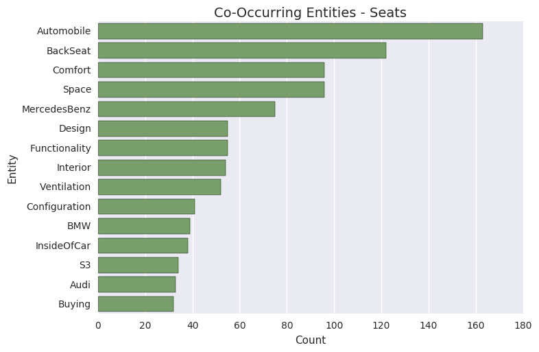
co_occurring_entities(entity, n=15, entity_type='')>>> absa.co_occurring_entities('Oil', n=5, >>> entity_type='feature_')
Feature
FuelConsumption    32
Power              28
Acceleration       10
Size                9
Body                6
Name: Count, dtype: int64
Also read about concept_frequency to see how entity_type can change output.
best_rated_entities(n=15, entity_type='')>>> absa.best_rated_entities(n=1)
Entity
X5    1.0
Name: Sentiment, dtype: float64
Also read about concept_frequency to see how entity_type can change output.
worst_rated_entities(n=15, entity_type='')>>> absa.worst_rated_entities(n=2)
Entity
Compartment   -1.0
Black         -0.81
Name: Sentiment, dtype: float64
Also read about concept_frequency to see how entity_type can change output.
-
>>> absa.surface_strings('ShockAbsorption')
{'ShockAbsorption': ['减震效果也非常好',
                     '减震效果和隔音效果也很好',
                     '减震效果也很好']}
-
>>> absa.entity_texts(['Room', 'FashionStyle'])
{'FashionStyle': ['外观很满意,外形稍显低调,但不缺乏时尚动感,整车的线条体现更是完整,看起来更为流畅,开眼角大灯我也比较喜欢,这车感觉就像一个穿着休闲西服的长腿欧巴,时而稳重,时而动感'],
 'Room': ['外观好看,室内舒适。']}
-
>>> absa.entity_sentiment({'Oil', 'Seats', 'Room'})
Entity
Oil      0.750002
Room     0.201
Seats    0.55238
Name: Sentiment, dtype: float64
Plotting
Most of the aggregation results from previous section can be rendered as a graph
using anacode.agg.plotting. The module knows how to plot three types
of graphs - horizontal barchart,
piechart and
word cloud.
Generally all results that have a meaningful graph representation can be plotted
using anacode.agg.plotting.barhchart(). Aggregation that do not have
graph representation currently are
nltk_textcollection,
make_idf_filter,
make_time_series,
main_category,
average_sentiment,
surface_strings and
entity_texts - all other aggregation
method results can be plotted as horizontal bar chart with
barhchart. Only
CategoriesDataset.categories aggregation method is
viable to be rendered as piechart and
ConceptsDataset.concept_frequencies is the only
aggregation method viable to be rendered as concept could.
>>> import matplotlib.pyplot as plt
>>> from anacode.agg import plotting
>>> concept_frequencies = concepts.concept_frequencies()
>>> plotting.concept_cloud(concept_frequencies)
>>> plt.show()
>>> from anacode.agg import plotting
>>> co_occuring = absa.co_occurring_entities('Seats')
>>> plotting.barhchart(co_occuring)